編碼
特徵編碼
使用時機:當特徵為類別型資料時,將其轉換為數值型資料以便於模型處理。
方法:將每個類別轉換為一個二進制特徵,適用於無序類別資料。
例子:將「顏色」特徵的「紅色」、「綠色」、「藍色」轉換為三個二進制特徵。
例子:國家特徵的「美國」、「加拿大」、「墨西哥」轉換為三個二進制特徵。
例子:模型無法直接處理類別變數,因此需要將其轉換為數值型資料。
不適合使用的情況:當類別數量過多時,會導致特徵維度過高,影響模型性能。有大量缺失值的類別特徵也不適合使用One Hot Encoding。
例子:如果「顏色」特徵有1000個不同的顏色,則會產生1000個二進制特徵,這會導致模型過於複雜。
例子:如果「國家」特徵有200個不同的國家,則會產生200個二進制特徵,這會導致模型過於複雜。
例子:如果「產品類別」特徵有500個不同的產品類別,則會產生500個二進制特徵,這會導致模型過於複雜。
範例程式碼:
                from sklearn.preprocessing import OneHotEncoder
                ohe = OneHotEncoder()

                # 指定要OHE編碼的columns list
                OHE_COL = ['col_1','col_2','col_3','col_4','col_5']
                # OHE轉換function
                # 輸入:DataFrame
                # 輸出:輸出一個包含指定column的OHE新的DataFrame
                def ohe_coding(d):
                    x_encoded = ohe.fit_transform(d[OHE_COL])
                    x_encoded = pd.DataFrame(x_encoded.toarray(), columns=ohe.get_feature_names_out(OHE_COL))
                    # 以df index進行編碼後table合併
                    x_encoded = pd.concat([pd.DataFrame({d.index.name:list(d.index)}),x_encoded],axis=1).set_index(d.index.name)

                    d2 = pd.concat([d, x_encoded], axis=1)
                    d2.drop(OHE_COL, axis=1, inplace=True)

                    return d2
特徵編碼
使用時機:當特徵為object時,將其轉換為數值型資料以便於模型處理。
方法:將data Series內所有值轉換為一個隨機數值,依據資料的出現順序編號。
注意:LabelEncoder為隨機編碥,若資料是大小順序關係,應使用OrdinalEncoder指定大小,或者使用.map()等函數自行指定為有大小關係的數值
範例程式碼:
                from sklearn.preprocessing import LabelEncoder
                le = LabelEncoder()

                # 假設 x 是一個 DataFrame,包含需要編碼的類別特徵
                for col in x.columns:
                    if x[col].dtype=='object':
                        x[col] = le.fit_transform(x[col])

                # 直接以map()操作賦值
                # 例:將data_col1 column中的資料值X_1 ~ X_3 改為編碼整數1,2,3
                df['data_col1'] = df['data_col1'].map({'X_1':1,'X_2':2,'X_3':3})
特徵編碼
使用時機:當特徵為object時,將其轉換為數值型資料以便於模型處理。
方法:與Label Encoding,差異就是可以指定資料(df['col_name'].unique())的大小順序
範例程式碼:
                # example features
                ordinal_features_df = {
                    'LotShape': ['IR3', 'IR2', 'IR1', 'Reg'],
                    'Utilities': ['ELO', 'NoSeWa', 'NoSewr', 'AllPub'],
                    'LandSlope': ['Sev', 'Mod', 'Gtl'],
                    'ExterQual': ['Po', 'Fa', 'TA', 'Gd', 'Ex'],
                    'GarageCond': ['NA', 'Po', 'Fa', 'TA', 'Gd', 'Ex']
                }

                # OE轉換function
                # 輸入:原資料dataframe, 欲編碼特徵唯一值大小排序dataframe
                # 輸出:修改過的原資料dataframe
                def oe_coding(data , feature_df):
                    categories = list(feature_df.keys())
                    encoder = OrdinalEncoder(categories=[feature_df[c] for c in categories])
                    data[categories] = encoder.fit_transform(data[categories])
                    return data

                #使用範例
                df2 = oe_coding(df, ordinal_features_df)
特徵編碼
使用時機:類別數量中等偏多(如10~1000個)、類別之間的統計資訊對目標有強關聯且資料量大,有足夠樣本來估計平均值
方法:將每個類別(category)替換成該類別在訓練集中對應的目標變數的平均值(常見用於回歸或分類問題)
優點:有效縮小高基數(high cardinality)類別維度,減少 one-hot encoding 的維度爆炸問題
缺點:容易 overfitting,特別是對樣本數少的類別、需要對訓練/驗證做資料泄漏(data leakage)處理且不適合類別與目標無明顯關聯時使用
範例程式碼:
                import pandas as pd
                import numpy as np

                # 建立一個模擬資料集
                data = {
                    'City': ['Taipei', 'Kaohsiung', 'Taipei', 'Taichung', 'Kaohsiung', 'Taipei', 'Taichung', 'Tainan', 'Taipei', 'Kaohsiung'],
                    'Income_USD': [50000, 65000, 52000, 58000, 68000, 51000, 60000, 55000, 53000, 67000]
                }
                df = pd.DataFrame(data)

                print("原始資料:")
                print(df)
                print("\n城市類別及對應的平均收入:")
                print(df.groupby('City')['Income_USD'].mean())

                from sklearn.model_selection import KFold

                # 定義要進行 Target Encoding 的類別特徵和目標變數
                categorical_feature = 'City'
                target_variable = 'Income_USD'

                # 初始化一個新的欄位來儲存編碼結果
                df['City_TargetEncoded'] = np.nan

                # ====================
                # 方法一:手動實現 Target Encoding (推薦在訓練集上執行,並應用於測試集)
                # 這裡為了展示方便,直接在整個資料集上計算,但實務中應避免在整個資料集上直接計算
                # ====================

                # 計算每個類別的目標平均值
                # 這個映射會用於將類別替換為對應的平均值
                target_mean_map = df.groupby(categorical_feature)[target_variable].mean()
                df['City_TargetEncoded_Manual'] = df[categorical_feature].map(target_mean_map)

                print("\n手動 Target Encoding 結果 (未平滑化):")
                print(df[[categorical_feature, target_variable, 'City_TargetEncoded_Manual']])

                # ====================
                # 方法二:引入平滑化 (Smoothing) 來處理低頻率類別,避免過度擬合
                # 當某些類別只出現幾次時,其目標平均值可能不夠穩定,容易導致過度擬合。
                # 平滑化的公式:(count * mean_category + global_mean * weight) / (count + weight)
                # 其中 weight 是一個超參數,用於平衡類別平均值和全局平均值。
                # ====================

                global_mean = df[target_variable].mean()
                print(f"\n全局目標平均值 (Global Mean): {global_mean:.2f}")

                # 設定平滑參數 (這個值需要根據資料集特性進行調整)
                smoothing_weight = 10

                # 計算每個類別的計數和平均值
                agg = df.groupby(categorical_feature)[target_variable].agg(['count', 'mean'])
                agg.columns = ['count', 'mean_category']

                # 應用平滑化公式
                agg['smoothed_mean'] = (agg['count'] * agg['mean_category'] + global_mean * smoothing_weight) / (agg['count'] + smoothing_weight)

                # 將平滑後的平均值映射回原始資料集
                df['City_TargetEncoded_Smoothed'] = df[categorical_feature].map(agg['smoothed_mean'])

                print("\n平滑化後的 Target Encoding 結果:")
                print(df[[categorical_feature, target_variable, 'City_TargetEncoded_Smoothed']])

                # ====================
                # 方法三:使用 K-Fold Cross-Validation 進行 Target Encoding (最佳實踐)
                # 這種方法可以有效避免資訊洩漏和過度擬合。
                # 在每個折疊中,我們使用訓練折疊的資料來計算編碼,然後應用於驗證折疊。
                # ====================

                kf = KFold(n_splits=5, shuffle=True, random_state=42) # 設定 KFold 參數

                df_encoded_cv = df.copy() # 複製一份資料來儲存交叉驗證的結果
                df_encoded_cv['City_TargetEncoded_CV'] = np.nan # 初始化為 NaN

                for fold, (train_index, val_index) in enumerate(kf.split(df)):
                    X_train, X_val = df.iloc[train_index], df.iloc[val_index]

                    # 計算訓練折疊的目標平均值 (帶平滑化)
                    train_global_mean = X_train[target_variable].mean()
                    train_agg = X_train.groupby(categorical_feature)[target_variable].agg(['count', 'mean'])
                    train_agg.columns = ['count', 'mean_category']
                    train_agg['smoothed_mean'] = (train_agg['count'] * train_agg['mean_category'] + train_global_mean * smoothing_weight) / (train_agg['count'] + smoothing_weight)

                    # 將編碼應用到驗證折疊
                    # 對於驗證折疊中訓練集未出現的類別,使用全局平均值填充
                    df_encoded_cv.loc[val_index, 'City_TargetEncoded_CV'] = X_val[categorical_feature].map(train_agg['smoothed_mean']).fillna(train_global_mean)

                print("\nK-Fold Cross-Validation Target Encoding 結果 (最佳實踐):")
                df_encoded_cv[[categorical_feature, target_variable, 'City_TargetEncoded_CV']]
特徵編碼
使用時機:特徵數量中至高且不想引入目標變數資訊(與 target 無關),適合用在預測與類別出現頻率有關的問題
方法:將每個類別值用它在資料中出現的「頻率」或「次數」來表示
缺點:如果類別頻率與目標無關,這個特徵幾乎是「噪聲」、不一定有可解釋性(頻率 ≠ 意義)且無法捕捉到類別與目標的直接關係
範例程式碼:
                import pandas as pd

                # 建立一個模擬資料集
                data = {
                    'City': ['Taipei', 'Kaohsiung', 'Taipei', 'Taichung', 'Kaohsiung', 'Taipei', 'Taichung', 'Tainan', 'Taipei', 'Kaohsiung', 'Taipei', 'Taipei', 'Taichung'],
                    'Product': ['A', 'B', 'A', 'C', 'B', 'A', 'D', 'C', 'A', 'B', 'D', 'C', 'A'],
                    'Sales': [100, 150, 120, 90, 160, 110, 80, 95, 130, 140, 105, 115, 85]
                }
                df = pd.DataFrame(data)

                print("原始資料:")
                print(df)

                # ====================
                # 方法一:Frequency Encoding (使用計數)
                # ====================

                # 計算每個城市出現的次數
                city_counts = df['City'].value_counts()
                print("\n城市出現次數:")
                print(city_counts)

                # 將 'City' 欄位替換為其計數
                df['City_Encoded_Count'] = df['City'].map(city_counts)

                # 計算每個產品出現的次數
                product_counts = df['Product'].value_counts()
                print("\n產品出現次數:")
                print(product_counts)

                # 將 'Product' 欄位替換為其計數
                df['Product_Encoded_Count'] = df['Product'].map(product_counts)

                print("\nFrequency Encoding (計數) 結果:")
                print(df[['City', 'City_Encoded_Count', 'Product', 'Product_Encoded_Count', 'Sales']])


                # ====================
                # 方法二:Frequency Encoding (使用頻率/比例)
                # ====================

                # 計算每個城市出現的頻率 (總計數的比例)
                city_frequencies = df['City'].value_counts(normalize=True)
                print("\n城市出現頻率:")
                print(city_frequencies)

                # 將 'City' 欄位替換為其頻率
                df['City_Encoded_Frequency'] = df['City'].map(city_frequencies)

                # 計算每個產品出現的頻率
                product_frequencies = df['Product'].value_counts(normalize=True)
                print("\n產品出現頻率:")
                print(product_frequencies)

                # 將 'Product' 欄位替換為其頻率
                df['Product_Encoded_Frequency'] = df['Product'].map(product_frequencies)

                print("\nFrequency Encoding (頻率) 結果:")
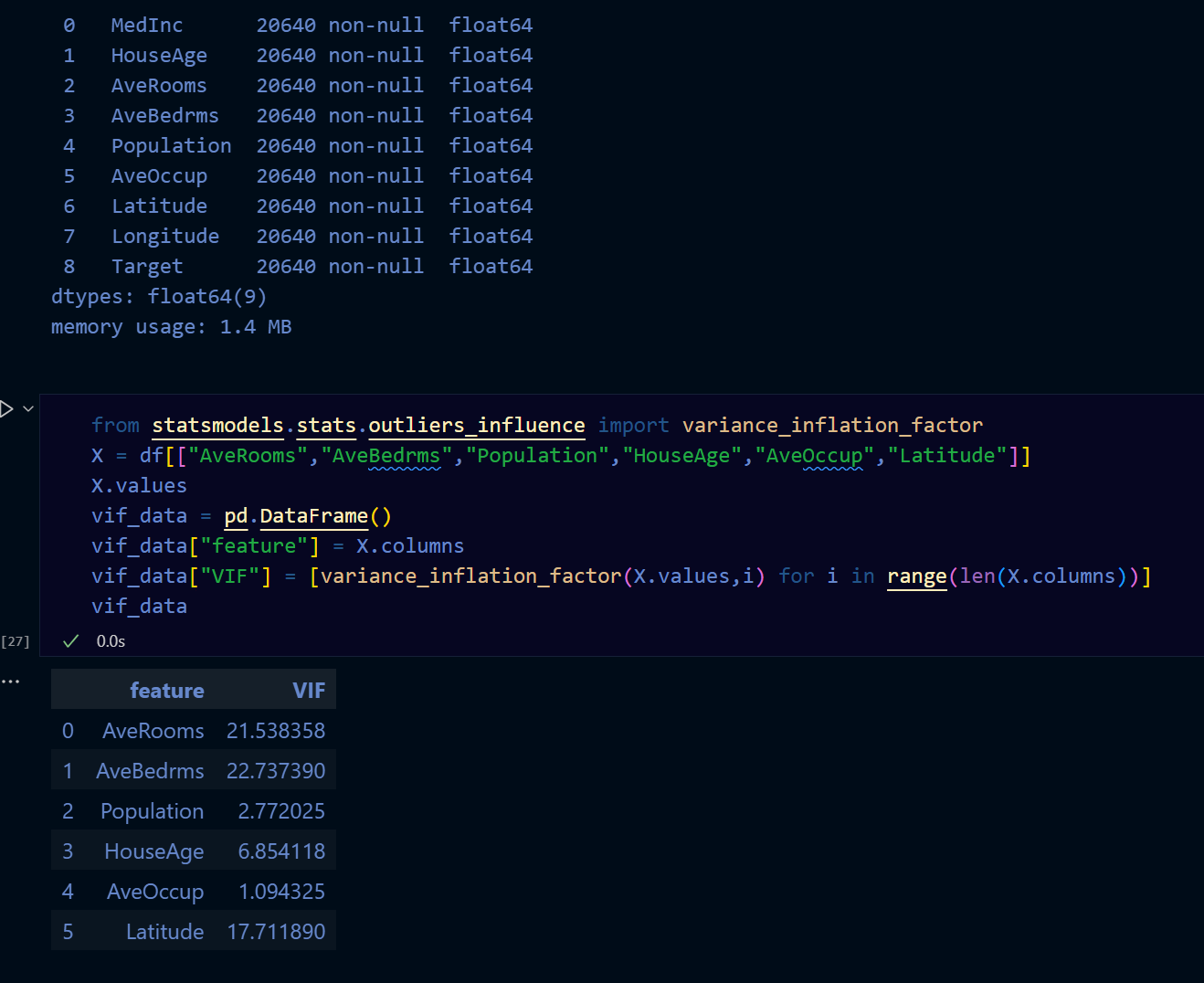
回歸VIF評估
VIF = 1 / (1 - R²)
其中R²是回歸模型的決定係數。
VIF值的解釋:
- VIF < 5:表示特徵之間的多重共線性問題不嚴重。
- 5 ≤ VIF < 10:表示特徵之間存在中等程度的多重共線性問題。
- VIF ≥ 10:表示特徵之間存在嚴重的多重共線性問題,可能需要考慮刪除或合併特徵。
VIF值的計算:
1. 對每個特徵,將其作為因變數,其他特徵作為自變數進行回歸分析。
2. 計算回歸模型的決定係數R²。
3. 使用VIF公式計算VIF值。
VIF值的意義:
VIF值用於評估特徵之間的多重共線性問題。當VIF值過高時,表示特徵之間存在較強的相關性,可能會影響模型的穩定性和解釋能力。
VIF值的範例:
假設有三個特徵A、B、C,計算得到的VIF值分別為:
- VIF(A) = 2.5
- VIF(B) = 6.8
- VIF(C) = 12.3
根據VIF值的解釋,可以得出以下結論:
- 特徵A的VIF值小於5,表示其與其他特徵之間的多重共線性問題不嚴重。
- 特徵B的VIF值介於5和10之間,表示其與其他特徵之間存在中等程度的多重共線性問題。
- 特徵C的VIF值大於10,表示其與其他特徵之間存在嚴重的多重共線性問題,可能需要考慮刪除或合併特徵。
特徵選取演算法
Sequential Feature Selection
原理:逐一加入特徵,並在每次加入一個特徵後計算模型分數,觀察是否有提升。
簡而言之,是一次加入一個特徵,檢查是否能提高分數
範例程式碼:
                from sklearn.feature_selection import SequentialFeatureSelector
                from sklearn.linear_model import LinearRegression

                # 假設 x 是特徵矩陣,y 是標籤
                model = LinearRegression() # 建立一個線性回歸模型
                sfs = SequentialFeatureSelector(model, n_features_to_select=5)
                x_sfs = sfs.fit_transform(x, y)  # y是標籤
Recursive Feature Elimination
原理:從全部特徵開始,每次移除對預測影響最小的特徵,然後重新評估模型的表現。
簡而言之,是一次移除一個特徵,檢查是否能提高分數
範例程式碼:
                from sklearn.feature_selection import RFE
                from sklearn.linear_model import LinearRegression

                # 假設 x 是特徵矩陣,y 是標籤
                model = LinearRegression() # 建立一個線性回歸模型
                rfe = RFE(model, n_features_to_select=5)
                x_rfe = rfe.fit_transform(x, y)  # y是標籤
Permutation Feature Importance
原理:對單一特徵的值進行隨機打亂(保持其他特徵不變),再觀察模型效能下降的幅度。
簡而言之,是隨機打亂一個特徵的值,檢查是否能提高分數
範例程式碼:
                from sklearn.inspection import permutation_importance
                from sklearn.ensemble import RandomForestClassifier

                # 假設 x 是特徵矩陣,y 是標籤
                model = RandomForestClassifier() # 建立一個隨機森林分類器
                model.fit(x, y)  # y是標籤
                result = permutation_importance(model, x, y, n_repeats=10, random_state=42)
                feature_importances = result.importances_mean
                feature_names = x.columns
                feature_importance_df = pd.DataFrame({'Feature': feature_names, 'Importance': feature_importances})
                feature_importance_df = feature_importance_df.sort_values(by='Importance', ascending=False)
                print(feature_importance_df)
特徵萃取
特徵萃取
屬於非監督式學習方法,主要用於資料降維。
公式:PCA = argmax(W^T * S * W / ||W||^2)
說明:將「很多個可能重複或相關的特徵」濃縮成「幾個更精簡、更有代表性的特徵」,用更少的維度來表達原本複雜的資料。
使用時機:當資料集的特徵數量過多,導致計算和存儲成本過高時,可以使用PCA進行降維。
範例程式碼:
                from sklearn.decomposition import PCA
                pca = PCA(n_components=2)
                x_pca = pca.fit_transform(x)
特徵萃取
屬於監督式學習方法,主要用於資料降維。
公式:LDA = argmax(W^T * S_B * W / W^T * S_W * W)
說明:其目標是將高維數據投影到低維空間,同時最大化類別之間的可分離性,並最小化類別內部的變異性。
使用時機:當資料集的特徵數量過多,導致計算和存儲成本過高時,可以使用LDA進行降維。
與PCA的區別:LDA是監督式學習方法,考慮了類別標籤,而PCA是非監督式學習方法,不考慮類別標籤。
範例程式碼:
                from sklearn.discriminant_analysis import LinearDiscriminantAnalysis as LDA
                lda = LDA(n_components=2)
                x_lda = lda.fit_transform(x, y)  # y是標籤
特徵縮放
特徵縮放
公式:X_scaled = (X - X_min) / (X_max - X_min)
使用時機:當特徵的值域差異較大時,使用MinMaxScaler可以將所有特徵縮放到相同的範圍(通常是0到1)。
特徵縮放
說明:用於將數據進行標準化,使其具有零均值和單位方差。
公式:X_scaled = (X - μ) / σ
使用時機:當特徵的分佈不均勻或存在異常值時,使用StandardScaler可以使數據更符合正態分佈,從而提高模型的性能。